Using NASA DEM data to create high resolution contour lines with QGIS
Recently, a few cycling buddies and I wanted to design our own cycling jerseys (a post about that whole process is in the making). Contours are a popular choice of theme for their simplicity and serve as an easy way of making the design unique and personal through choice of the geographical location.
Using SwissTopo
Finding ready-made contour imagery was surprisingly difficult.
The Federal Office of Topography Switzerland SwissTopo has a fantastic high resolution interactive map with lots of different datasets.
And even though it has different height models, there are no ready-made contour images. I’m sure one could download some of the datasets and work on that further.
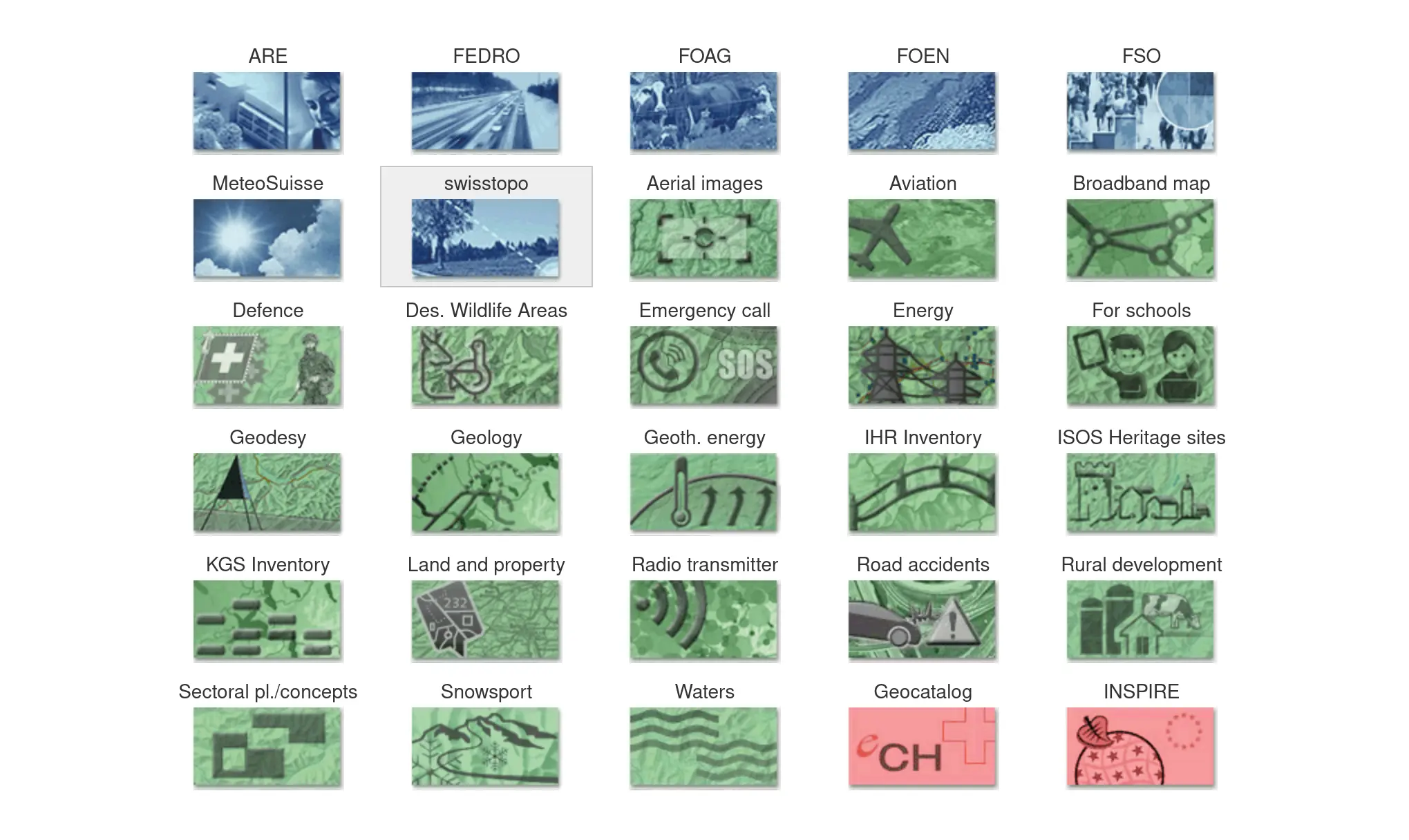
The closest thing (artistically) I could find to contour line was the Gravimetric Atlas
with a little imagemagick magic, I could transform this into a low quality version
Of course this has nothing to do with contours and it doesn’t allow for any customisation. Anyway, it is a cool resource that I wanted to share.
Using QGIS
Instead of relying on pre-made contour images we can try to make our own; this has the advantage that we can configure parameters as such the height between contour lines, colours, line thickness.
QGIS is a program with which one can manipulate map data; but before we get onto using that, we need to source the Digital Elevation Model (DEM) data from which we can produce contour lines.
Downloading NASA’s data
NASA offers many different elevation model datasets. One of the highest resolution datasets currently available is the NASA Shuttle Radar Topography Mission Global (SRTMGL1) dataset which is accurate up to 1-arc second (~30m). Another 1 arc-second resolution dataset is the Terra Advanced Spaceborne Thermal Emission and Reflection Riometer (ASTER) Global Digital Elevation Model (GDEM) version 3.
After creating a free account, this data can be downloaded by the public through the earthdata portal. If the link doesn’t work, search for “SRTMGL1” in the main search field of search.earthdata.nasa.gov. Under the “NASA Shuttle Radar Topography Mission Global 1 arc second V003” section, there are ~15,000 “granules” each with a title of the form
N<North Coordinate>E<East Coordinate>.SRTMGL1.hgt.zip
S<South Coordinate>E<East Coordinate>.SRTMGL1.hgt.zip
N<North Coordinate>W<West Coordinate>.SRTMGL1.hgt.zip
S<South Coordinate>W<West Coordinate>.SRTMGL1.hgt.zip
for example
N47E008.SRTMGL1.hgt.zip
for Zurich. Note the search function for Granule ID(s) searches for exact
matches, so use the wildcard * character.
The downloaded granule will be in the form of a zip archive with a title like
N47E008.SRTMGL1.hgt.zip. We don’t need to worry about unzipping this because
QGIS will do this automatically for us.
Downloading can be automated in a script
EARTHDATA_USERNAME=<EARTHDATA_USERNAME>
EARTHDATA_PASS=<EARTHDATA_PASS>
LOCATION=N47E008
wget --user="$EARTHDATA_USERNAME" --password="$EARTHDATA_PASS" \
  "https://e4ftl01.cr.usgs.gov/DP133/SRTM/SRTMGL1.003/2000.02.11/$LOCATION.SRTMGL1.hgt.zip"
This makes downloading many granules at once a lot easier.
Creating Contours
Now that we have the elevation data, we can easily import this data into QGIS.
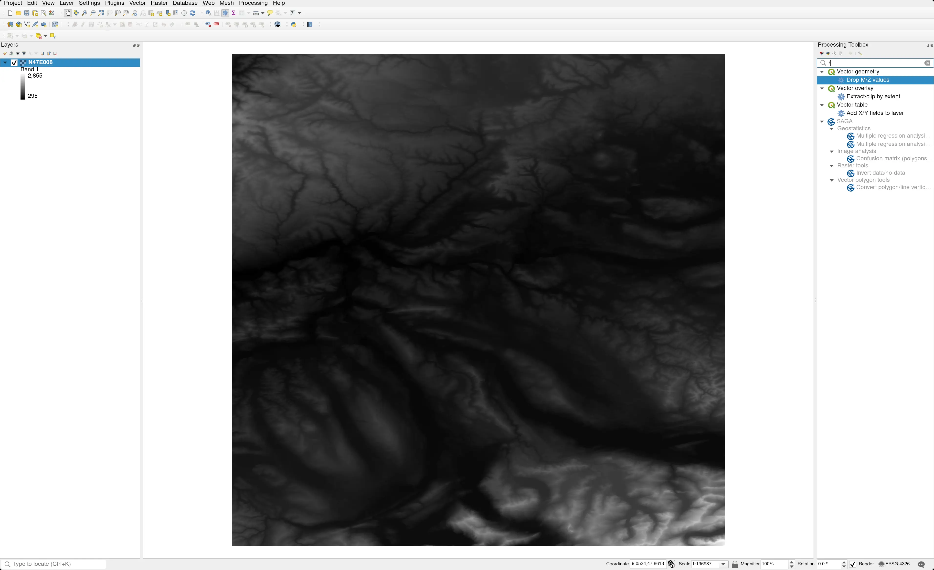
First open QGIS and find the downloaded hgt.zip file in the file browser.

(See how QGIS automatically extracted the zip file). Now select the hgt file
within the zip and you should see something like
Now under Raster > Extraction > Contour we get the menu
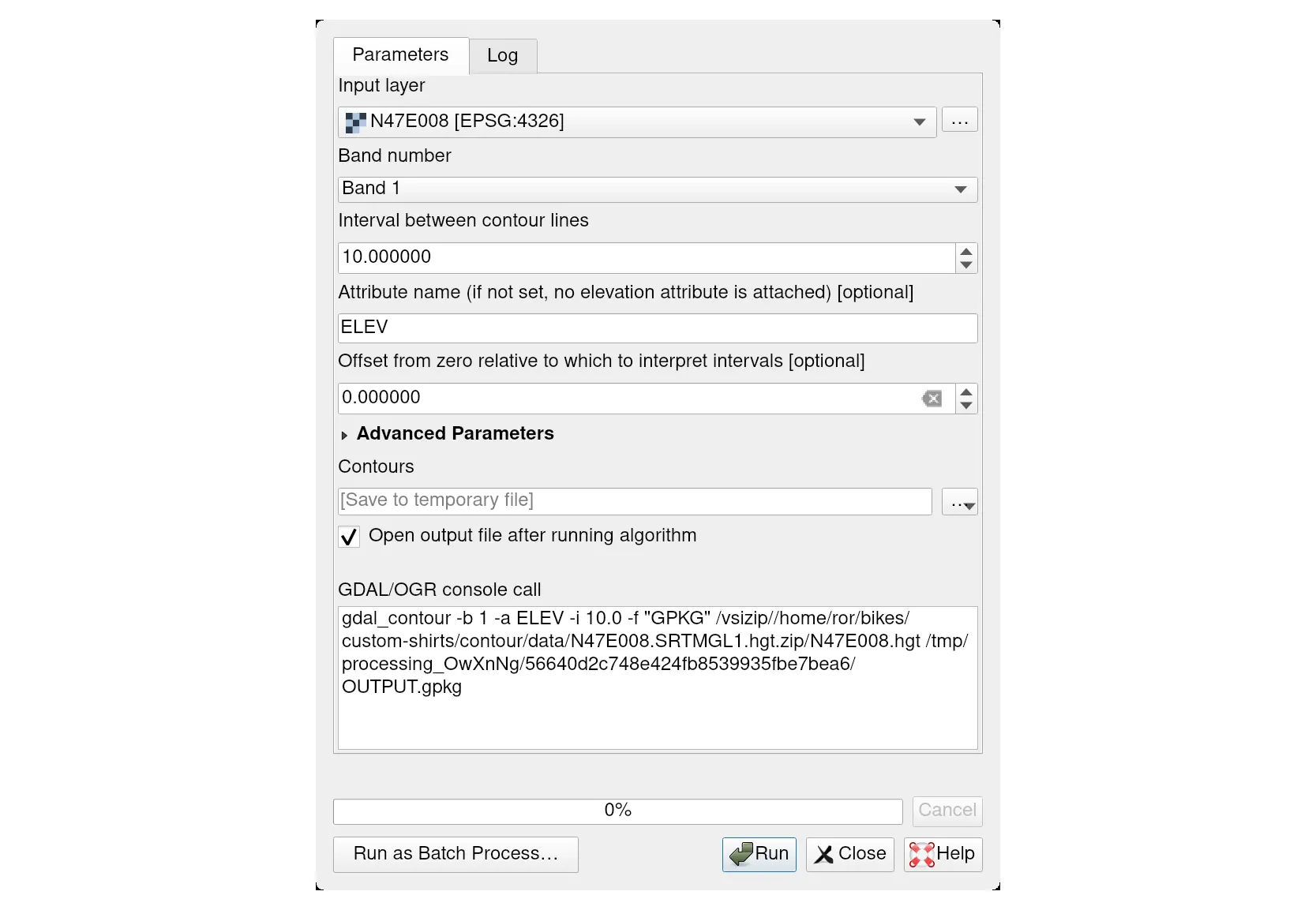
Changing the interval to 50m and clicking Run will yield
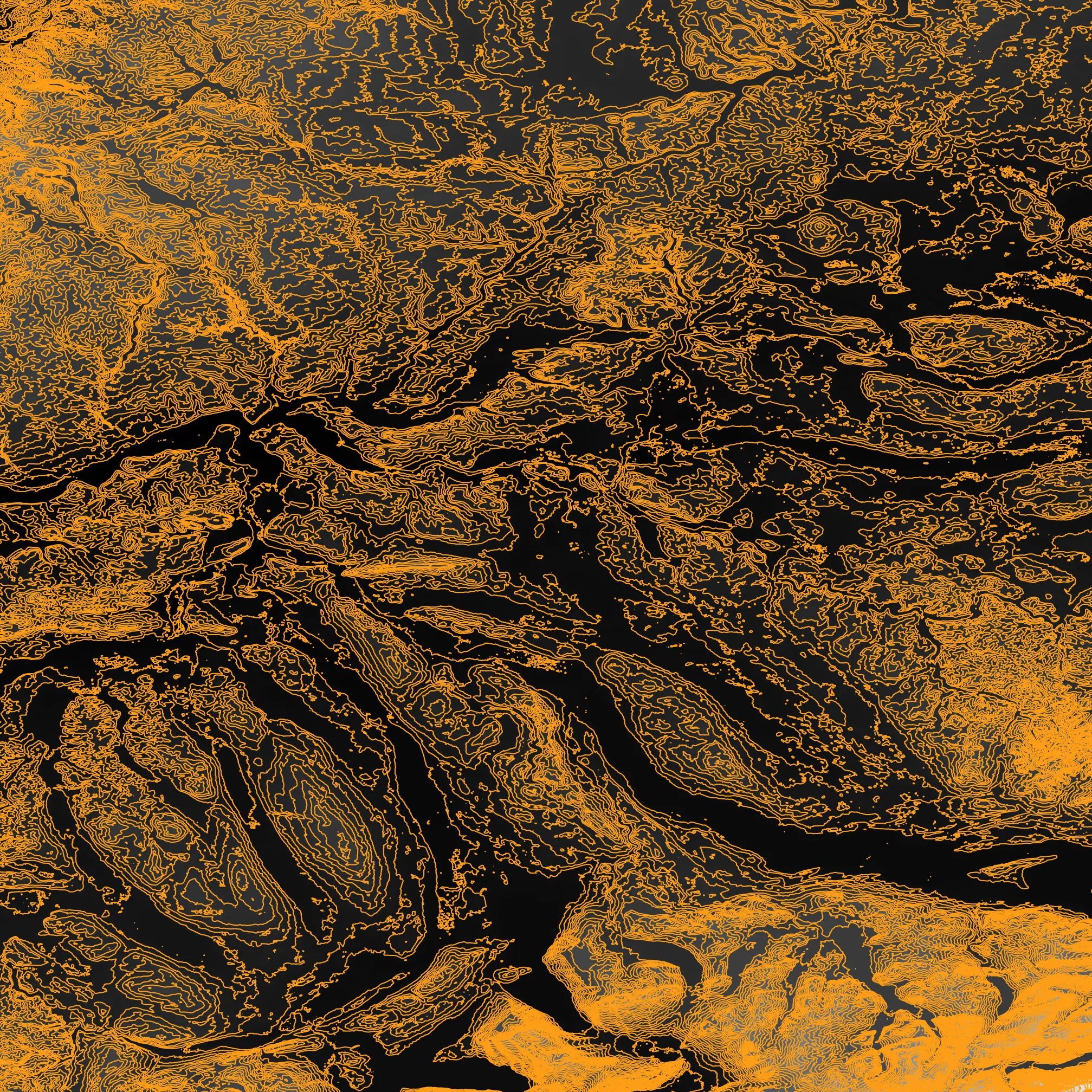
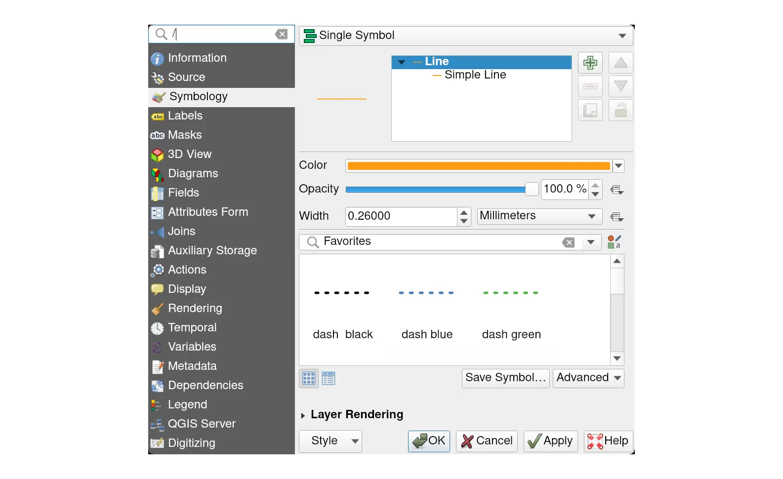
We can deselect the background and change the colour of the contours by double clicking the contour layer
to get
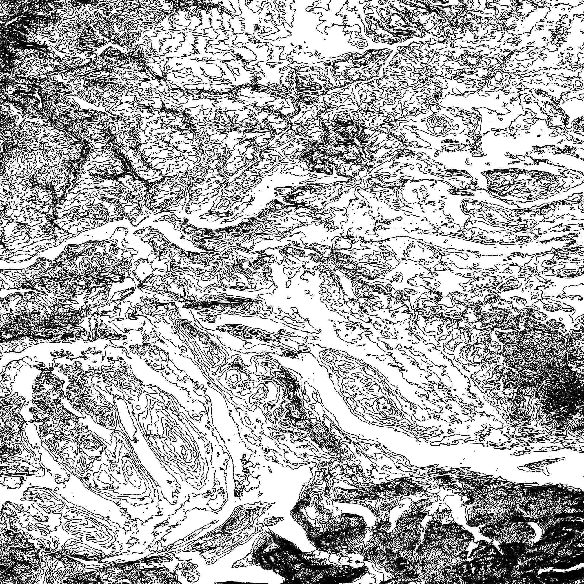
Whilst these contours are exactly geographically correct, they aren’t so aesthetically pleasing. Especially if they are going to be printed on a shirt. So we may want to ‘smooth out’ the data to make the lines flow a little cleaner.
Smoothing the contour lines
Even if we were able to smooth the contour lines themselves, we would still get small islands all over the place.
To solve this problem, we need to smooth the underlying data. That is, the hgt
file that we downloaded. Theoretically, this should be possible directly in QGIS
using the Gaussian filter from the processing toolbox
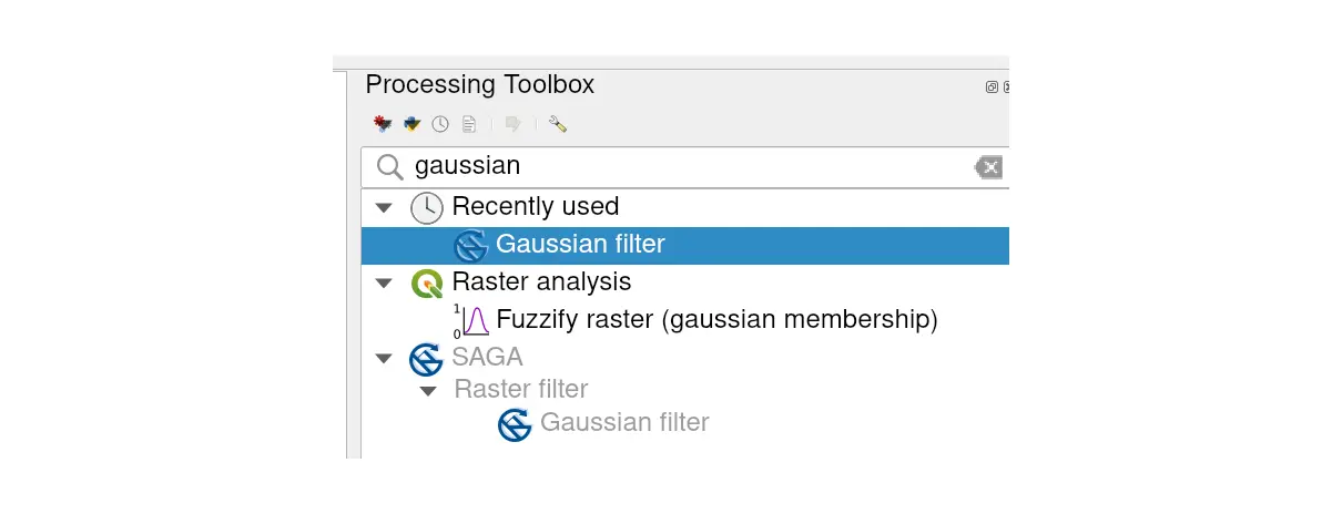
(you may have to install “SAGA GIS” before this filter becomes available in
QGIS. Available in Ubuntu as saga and the Archlinux User Repository (AUR) as
saga-gis )
however, my version of SAGA is not compatible with my version of QGIS
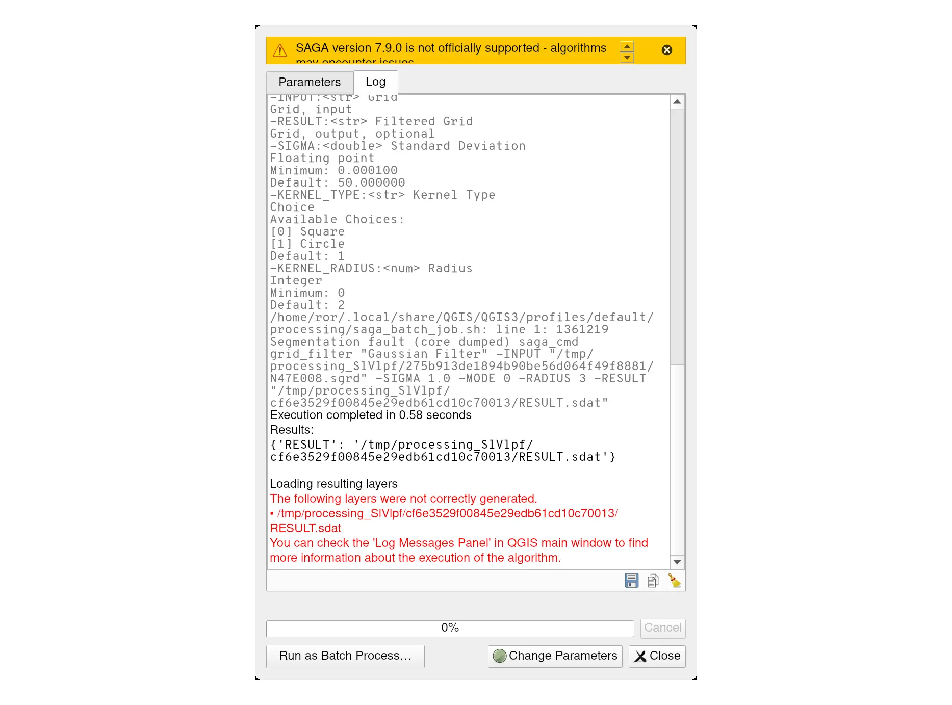
The output of the error is quite handy though, we can see what command QGIS
tried to execute, and simply try this ourselves in the console. Before we do
that though, we need to extract the .hgt.zip file to just the .hgt file.
SIGMA=50
KERNEL=100
ORIGINAL=$LOCATION.hgt
SMOOTHED=$LOCATION-s$SIGMA-r$KERNEL.sdat"

saga_cmd grid_filter "Gaussian Filter" -INPUT "$ORIGINAL" -SIGMA "$SIGMA" -KERNEL_TYPE 0 -KERNEL_RADIUS "$KERNEL" -RESULT "$SMOOTHED"
Note that smoothing can take a very long time (~1 hour). So I have provided a
small test grid showing how different values of $SIGMA and $RADIUS will give
us different types of smoothing
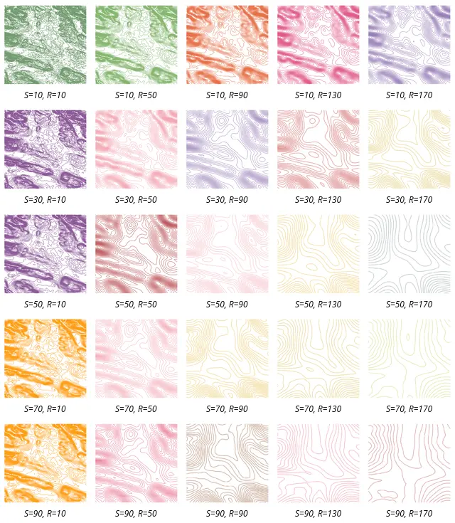
However, it is likely, that some trial and error will be required.
Creating Contours (Part 2)
I will continue using N47E008 smoothed with SIGMA=50 and RADIUS=100.
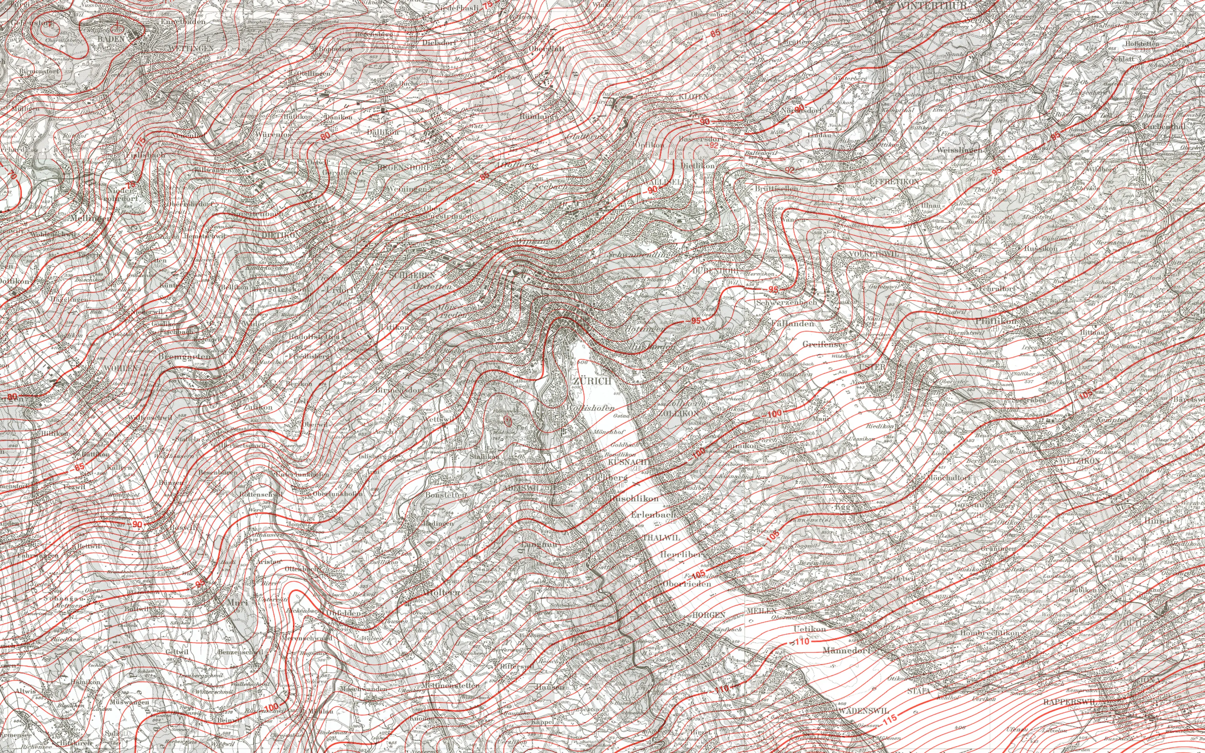
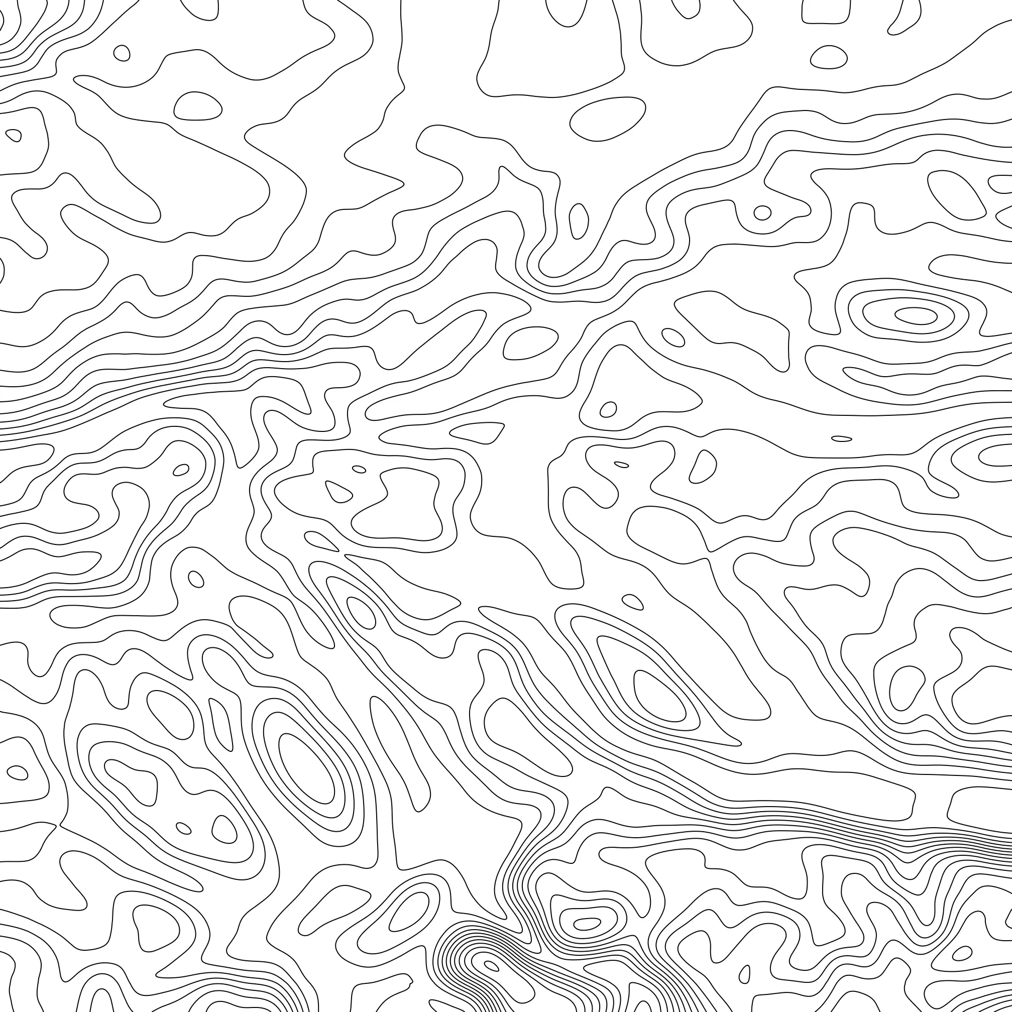
We can create different types of graphics now
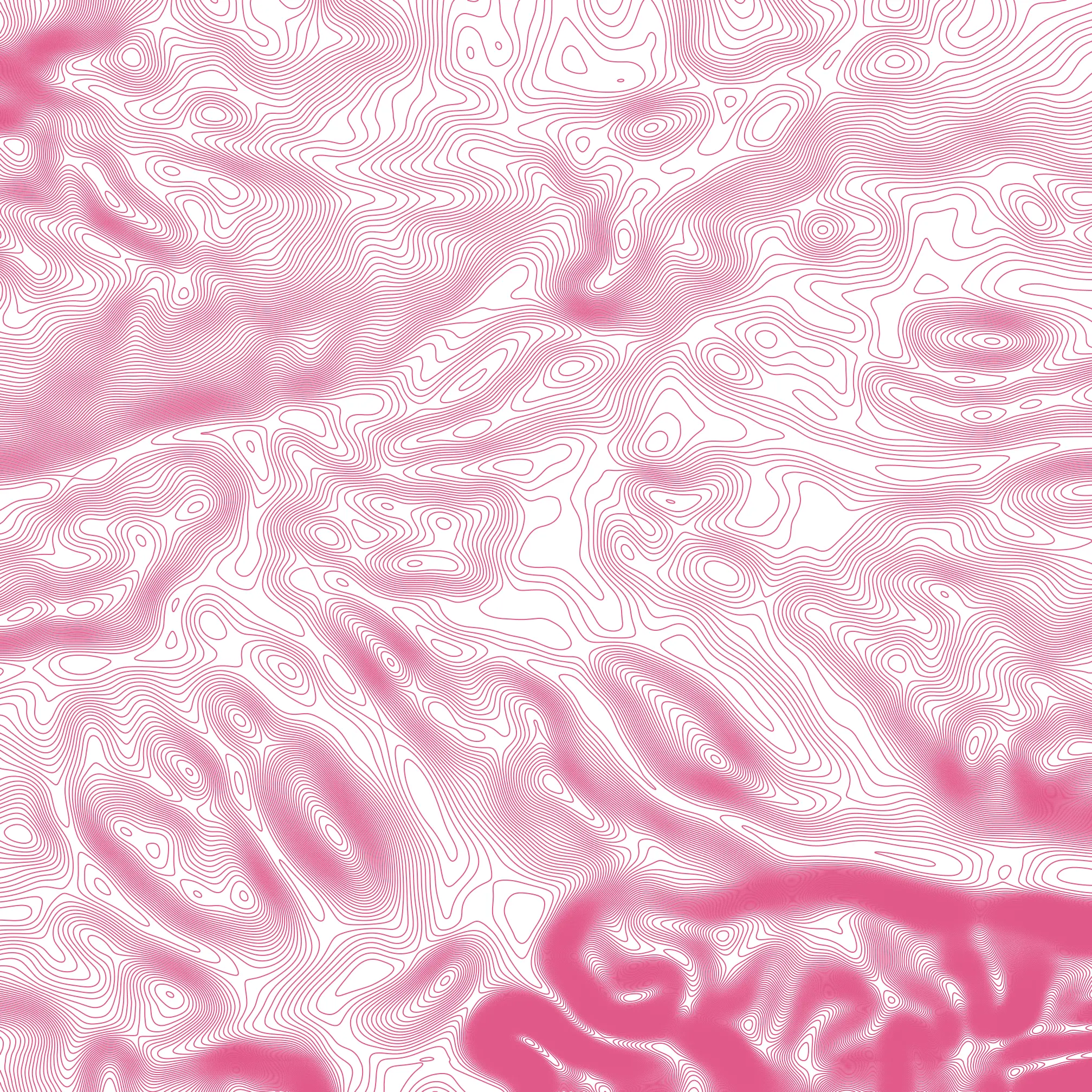
10m Elevation Differences
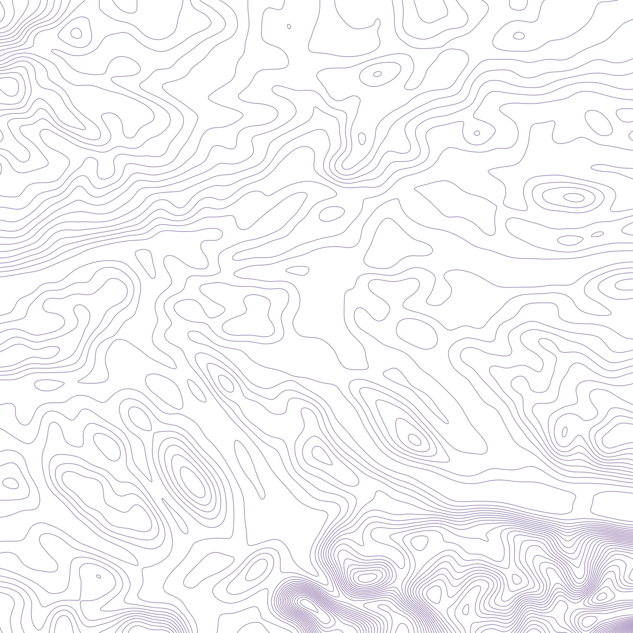
50m Elevation Differences
100m Elevation Differences
By adding a thicker set of contours every 50m to the 10m contour lines, we get this kind of graphic
25m and 75m Elevation Differences
It is possible to add labels and other features. This is described in great detail in this video by “Open Source Options”. Although this has limited application since we have smoothed the data, making it geographically incorrect; although, having elevation labels may fit the “contour line aesthetic”.
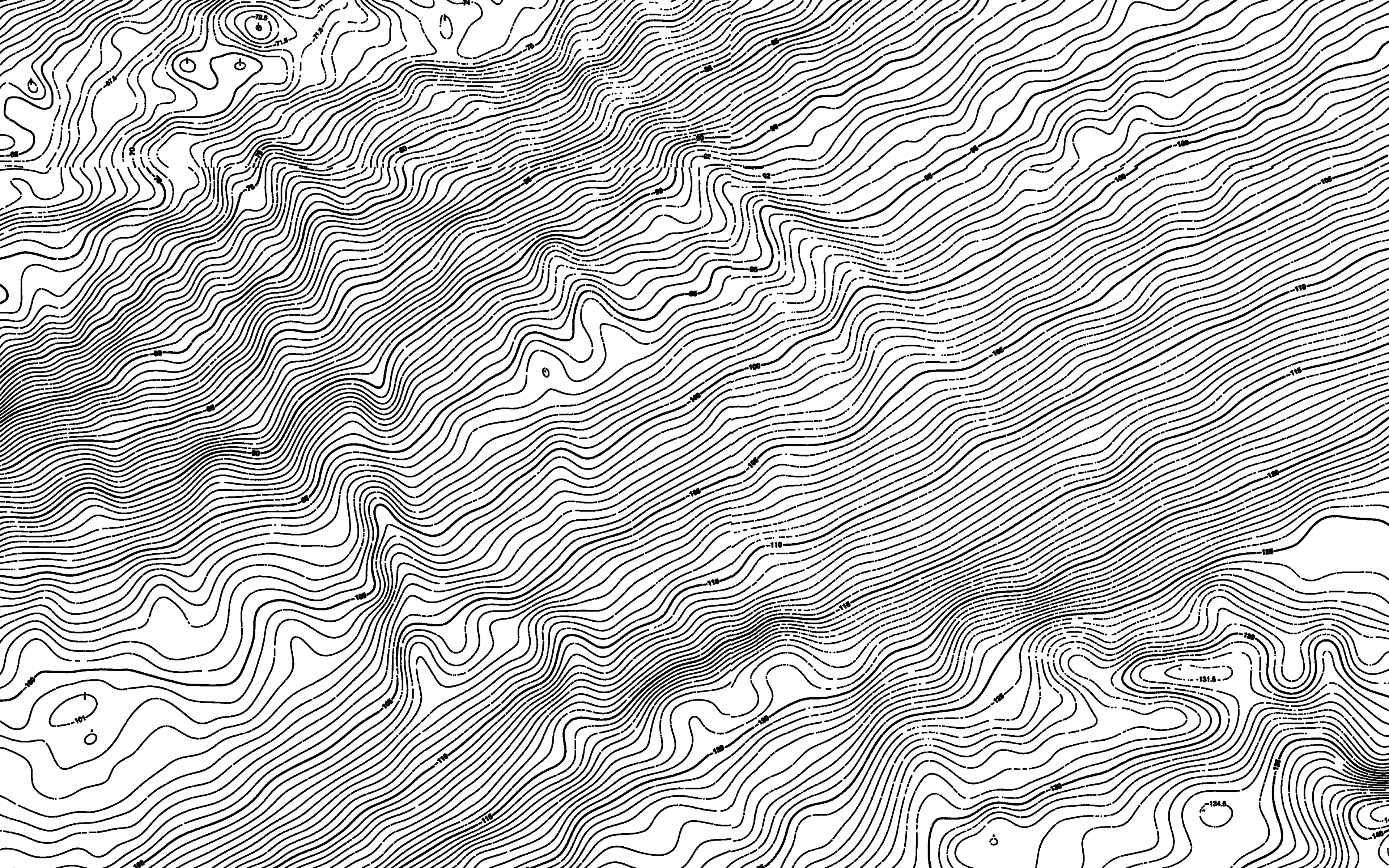
Often however, drawing contour lines a fixed distance apart creates a
combination of crowded pockets and sparse planes. We can fix this, by drawing
contour lines at exponential height intervals. That is, for a given base $b$,
draw contour lines at heights $b^1, b^2, b^3, \ldots$. I had to do some trial
and error with different bases, and settled on 1.1.
However, since Zurich as a whole is at around 400m above sea level, the
differences between 400m and 500m aren’t that obvious: the difference in
elevation between contour lines is increasing, meaning that there aren’t many
contour lines between 400m and 500m. gdal_contour has an -OFFSET option
which allows one to specify what we consider to zero (relative) elevation.
Ultimately, this will cause contour lines to be drawn at $C + b^1, C + b^2, C +
b^3, \ldots$ where $C$ is the offset constant.
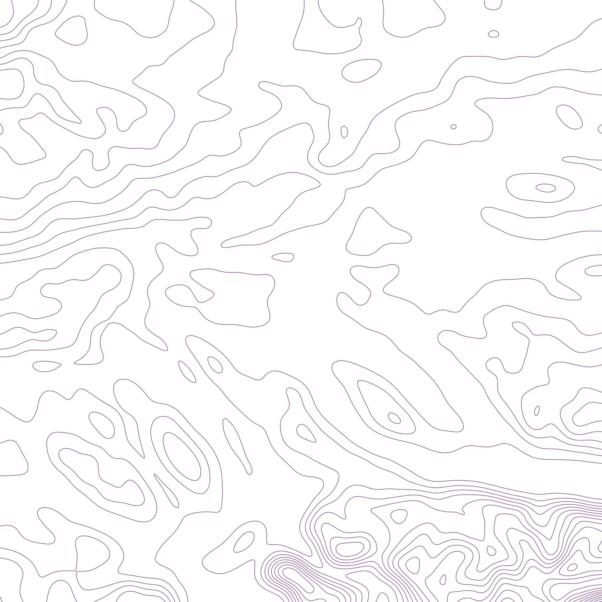
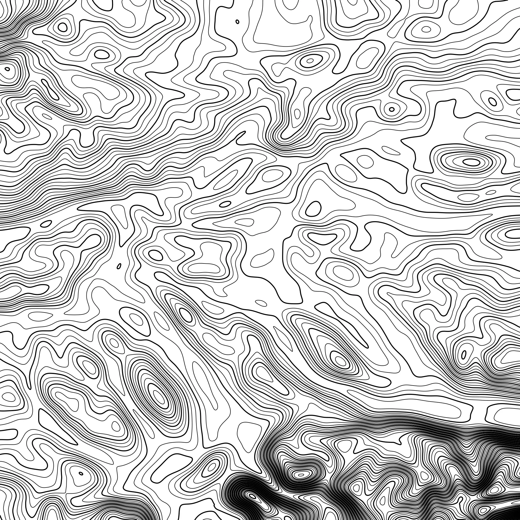
Exponential with base 1.1 no offset
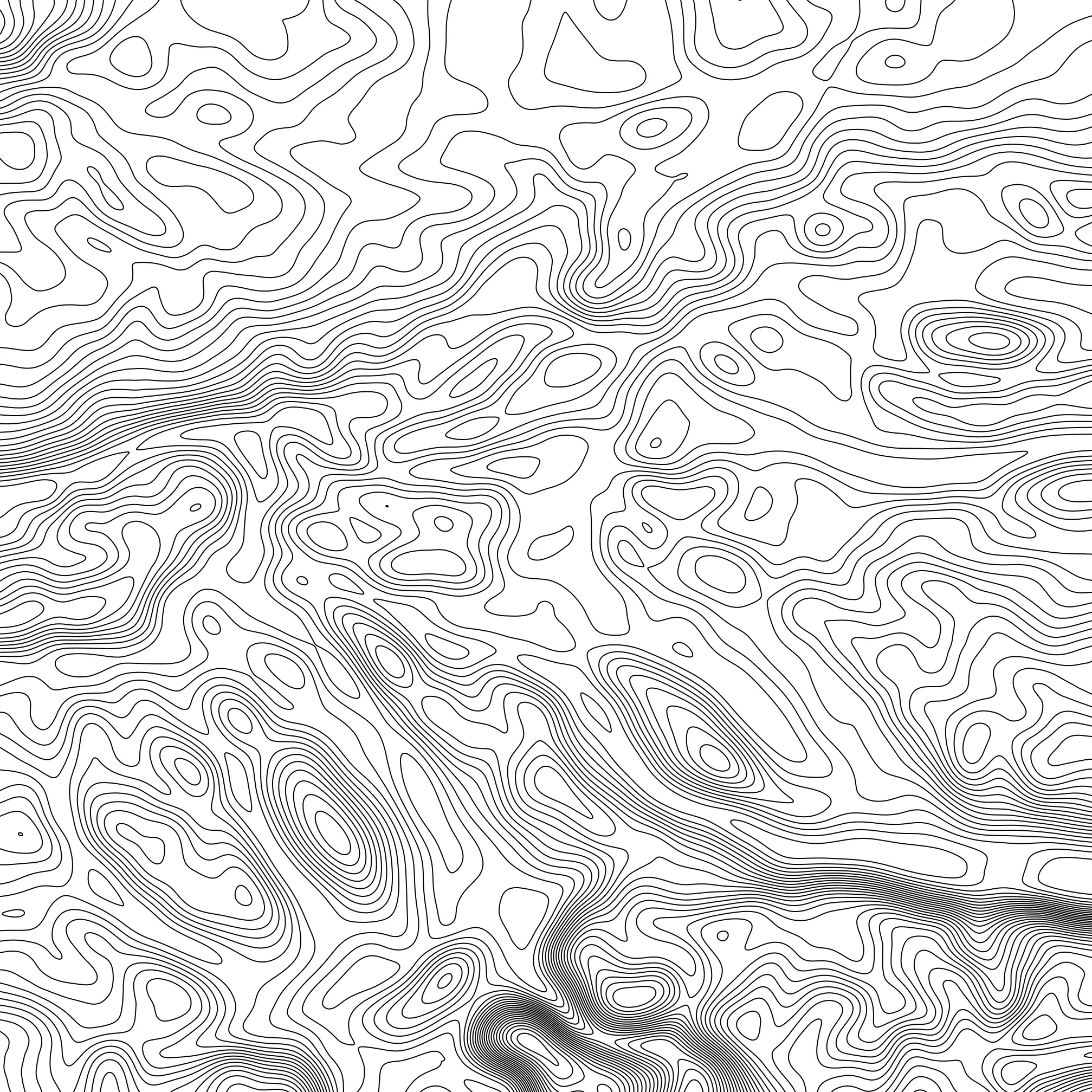
Exponential with base 1.1 offset 400m
With this option, smaller deviations in the flatter areas are still visible without crowding hilly areas many contour lines.
Automating almost everything
We can automate the entire process quite easily with two scripts found on my GitHub account.
The bash script handles downloading the data from NASA, smoothing the data,
and then producing the contour files.
The python script takes the contour files and actually draws them into a png
image.